hfsdoc

@@@@@@@@@@@@@@@@@@@@@@@@@@@@@@@@@@@@@@@@@@@@@@@@@@@@@@@@@@@@@@@@@@@@@@@@@@@@@@@@@@@@@@@@@@@@@@@@@@@@@@@@@
@                                                                                                       @
@    @@     @@ @@@@@@@@ @@@@@@@@     @@@@@@@@    @@@     @@@@@@  @@@@@@@@     @@@@@@  @@@@ @@     @@    @
@    @@     @@ @@       @@     @@    @@         @@ @@   @@    @@    @@       @@    @@  @@  @@@   @@@    @
@    @@     @@ @@       @@     @@    @@        @@   @@  @@          @@       @@        @@  @@@@ @@@@    @
@    @@@@@@@@@ @@@@@@   @@@@@@@@     @@@@@@   @@     @@  @@@@@@     @@        @@@@@@   @@  @@ @@@ @@    @
@    @@     @@ @@       @@           @@       @@@@@@@@@       @@    @@             @@  @@  @@     @@    @
@    @@     @@ @@       @@           @@       @@     @@ @@    @@    @@       @@    @@  @@  @@     @@    @
@    @@     @@ @@@@@@@@ @@           @@       @@     @@  @@@@@@     @@        @@@@@@  @@@@ @@     @@    @
@                                                                                                       @
@@@@@@@@@@@@@@@@@@@@@@@@@@@@@@@@@@@@@@@@@@@@@@@@@@@@@@@@@@@@@@@@@@@@@@@@@@@@@@@@@@@@@@@@@@@@@@@@@@@@@@@@@

Table of Contents

• Introduction
• Quick Start
• General Concept
• Code
• Getting Started
• Configuration Setup
• Running on Virgo
• Tools
• Demos
  • Generator Only
  • Geometric Acceptance
  • PID Templates
  • Secondary Vertex
  • Background Study
  • Using Variables
• Appendix

Demos

In the folder cfg are several example configuration files addressing different aspect and possibilities to run HepFastSim. In the following some of the demos are discussed a bit more detailed.

Generator only

Back to TOC

It is possible to completely skip the simulation part (acceptance cuts, efficiency, smearing, combinatorics, …) and use HepFastSim only as a generator tool for decay patterns. This is demonstrated in the configuration file cfg/demo_gen.cfg.

OPT  ;; nmc : print=5000 : hconf=450,3

GEN  ;; phsp : ecm=5,0.01 : reaction=anti-p-,p+ : fixtarget 
GEN  ;; phsp : c=1 : f=0.5 : dec = pbarpSystem -> omega pi+ pi- ; omega -> pi+ pi-  
GEN  ;; box  : c=2 : f=0.5 : p=1,2 : tht=22,140 : pdg=pi+- : mult=1

# simple p vs theta plot from box generator (chan==2)
HIST ;; tree=nmc : cut=chan==2 : hist=0,3,0,180 : var=p,tht*57.3 : opt=box : title=box generator;p [GeV/c];\theta [deg]

# generated omega mass from ppbar -> omega (-> pi+ pi-) pi+ pi-
HIST ;; tree=nmc : cut=chan==1 : hist=0.70,0.86 : var=m[1] : divx=505 : title=generated omega mass;m(\omega) [GeV/c^{2}]

# Dalitz plot of omega pi+ pi- (the needed masses can be computed from the 4-vector informations)
HIST ;; tree=nmc : cut=chan==1&&abs(m[1]-0.782)<0.3 : hist=0,26,0,26 : ...
        var=((e[1]+e[4])^2-(px[1]+px[4])^2-(py[1]+py[4])^2-(pz[1]+pz[4])^2),((e[1]+e[5])^2-(px[1]+px[5])^2-(py[1]+py[5])^2-(pz[1]+pz[5])^2) : ...
        title=Dalitz plot;m^{2}_{\omega\pi^{+}} [GeV^{2}/c^{4}];m^{2}_{\omega\pi^{\minus}} [GeV^{2}/c^{4}] 

Explanation:

• In the line OPT we need to enable the MC tree generation by setting nmc, from which we want to generate histograms
• The three GEN statements configure two generators:
  • the phsp generator with a initial reaction and the decay pbar p -> omega pi+ pi- (channel c=1)
  • the box generator generating single pions (mult=1) with p = 1 .. 2 GeV/c and theta = 22° .. 140° (channel c=2)
• Three histograms are created:
  • p vs theta coverage of the box generator
  • the generated mass of omega(782) from decays pbar p -> omega (-> pi+ pi-) pi+ pi-
  • the omega pi+ pi- Dalitz plot (the expressions for the square masses need to be computed from the 4-vectors)

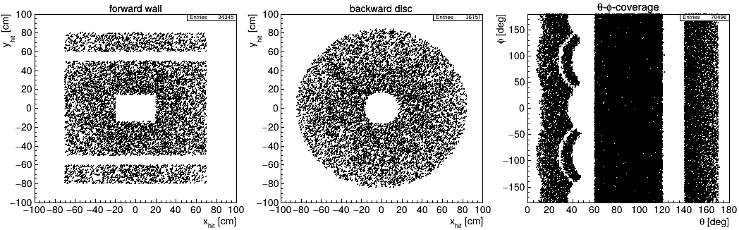
Geometric Acceptance

Back to TOC

Since it is possible to setup detector spatial coverage in different ways, the file cfg/demo_acc.cfg demonstrates and visualizes some possibilities.

# ----- generator ------
GEN ;; box : p=2,2 : tht=0,180 : costht : pdg=pi+  : mult=1

# ----- detectors ------
TRK  ;;  name = trk1 : dist=100  : wall=70,50,20,15   # forward wall center (140x100 cm with hole of 40x30cm) 
TRK  ;;  name = trk2 : dist=100  : wall=70,10,,,,70   # forward wall top    (140x20 cm, shifted up by 70cm)
TRK  ;;  name = trk3 : dist=100  : wall=70,10,,,,-70  # forward wall bottom (140x20 cm, shifted down by 70cm)
TRK  ;;  name = trk4 : dist=-100 : tht=140,170        # backward disc (hole for 170 deg < theta < 180 deg)
TRK  ;;  name = trk5 : dist=65   : tht=60,120         # barrel

# ----- reconstruction ------
REC  ;;  store(trk, ntp0) = evt,cand

# ----- plots ------
HIST ;; tree=ntp0 : hist=100,-100,100,100,-100,100 : opt=box : cut=xmct&&xtht<1.57 : var=(100-xz)*tan(xtht)*cos(xphi)+xx,(100-xz)*tan(xtht)*sin(xphi)+xy : title=forward wall;x_{hit} [cm];y_{hit} [cm] 
HIST ;; tree=ntp0 : hist=100,-100,100,100,-100,100 : opt=box : cut=xmct&&xtht>1.57 : var=(100-xz)*tan(xtht)*cos(xphi)+xx,(100-xz)*tan(xtht)*sin(xphi)+xy : title=backward disc;x_{hit} [cm];y_{hit} [cm]
HIST ;; tree=ntp0 : hist=90,0,180,90,-180,180      : opt=box : var=xtht*57.3,xphi*57.3 : title=\theta-\phi-coverage;\theta [deg];\phi [deg]

Explanation:

• Setup of a very simple box generator with mono-energetic single pions with p = 2 GeV/c in full theta range
• Define five detector components:
  • trk1: central foward wall of size 140x100cm with a hole 40x30cm at z = 100cm
  • trk2: upper forward wall of size 140x20cm shifted up by 70cm at z = 100cm
  • trk3: lower forward wall of same size shifted down by 70cm at z = 100cm
  • trk4: backward disc defined by angular range theta = 140° .. 170° at z = -100cm
  • trk5: barrel parallel to z-axis defined by angular range theta = 60° .. 120° with radius r = 65cm
• Store tree with tracks candidates only
• Generate three plots:
  • Hit map of all three foward walls by computing track positions at z = 100cm from theta, phi
  • Hit map of backward disc by computing track positions at z = -100cm from theta, phi
  • Hit map theta vs phi for all detectors

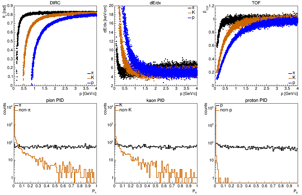
PID Templates

Back to TOC

Here we try and test some of the PID templates: DIRC (Detection of Internally Reflected Cherenkov light), the dE/dx and the time-of-flight. We plot the simulated quantities and the resultant total PID probabilities (line numbers below are for explanation only).

01: # ===== Overall options ===== 
02: OPT  ;;  rndseed=123 : verbose=1 : hconf=400,3 : pidmode=chi2 : nostat : legwid=0.1 : legmarg=0.5 : legtxt=0.05 : print=5000 : hopt=hist scat : errlvl=3
03: 
04: # ===== Generators ===== 
05: GEN  ;;  box : p=0.1,4 : tht=10,150 : pdg=pi+-, K+-, p+ cc : mult=1 
06: 
07: # ===== Trees/Reco ===== 
08: REC  ;;  store(trk,ntp0) = evt,cand
09: 
10: # ===== Detectors ===== 
11: TRK  ;;  name=trk  : tht=20,140          # Tracking detector
12: PID  ;;  name=drc  : tht=20,140 : dircb  # DIRC template (barrel)
13: PID  ;;  name=dedx : tht=20,140 : dedx   # dE/dx template (STT)
14: PID  ;;  name=tof  : tht=20,140 : tofb   # ToF template (barrel)
15: 
16: # ===== Histograms ===== 
17: HIST ;; tree=ntp0 : var=xp, xdrc  : hist=100,0,4,100,0,0.9 : cut=abs(xtrpdg)==211 : leg=\pi : legpos=br : title=DIRC;p [GeV/c];\theta_{c} [rad]
18: HIST ;; cut=abs(xtrpdg)==321 : leg=K   
19: HIST ;; cut=abs(xtrpdg)==2212 : leg=p  
20: 
21: HIST ;; tree=ntp0 : var=xp, xdedx : hist=100,0,4,100,2,20 : cut=abs(xtrpdg)==211 : leg=\pi : legpos=tr : title=dE/dx;p [GeV/c];dE/dx [keV/cm]
22: HIST ;; cut=abs(xtrpdg)==321 : leg=K  
23: HIST ;; cut=abs(xtrpdg)==2212 : leg=p 
24: 
25: HIST ;; tree=ntp0 : var=xp, xtof  : hist=100,0,4,100,0,1.2 : cut=abs(xtrpdg)==211 : leg=\pi : legpos=br : title=TOF;p [GeV/c];\beta_{TOF}
26: HIST ;; cut=abs(xtrpdg)==321 : leg=K   
27: HIST ;; cut=abs(xtrpdg)==2212 : leg=p  
28: 
29: HIST ;; tree=ntp0 : var=xpidpi : hist=0,1 : cut=abs(xtrpdg)==211 : leg=\pi : logy : title=pion PID;P_{\pi}
30: HIST ;; cut=abs(xtrpdg)!=211 : leg=non-\pi
31: 
32: HIST ;; tree=ntp0 : var=xpidk : hist=0,1 : cut=abs(xtrpdg)==321 : leg=K : logy : title=kaon PID;P_{K}
33: HIST ;; cut=abs(xtrpdg)!=321 : leg=non-K
34: 
35: HIST ;; tree=ntp0 : var=xpidp : hist=0,1 : cut=abs(xtrpdg)==2212 : leg=p : logy : title=proton PID;P_{p}
36: HIST ;; cut=abs(xtrpdg)!=2212 : leg=non-p

Explanation:

• (01) : Define general options (errlvl=3 suppresses the SCAT is deprecated output)
• (05) : Setup of a box generator generating pions, kaons, protons over large p- and theta range
• (08) : Store a TTree with the single tracks (no combinatorics)
• (11) : Setup tracking detector to cover full phase-space (we need detected tracks for PID information)
• (12-14) : Define PID detectors based on the templates dircb (barrel DIRC), dedx and tofb (barrel ToF)
• (17-27) : Generate histograms of PID info (xdrc, xdedx, xtof) vs. momentum for the three different particle species (pi, K, p)
• (29-36) : Generate histograms of PID probability for the three particle species

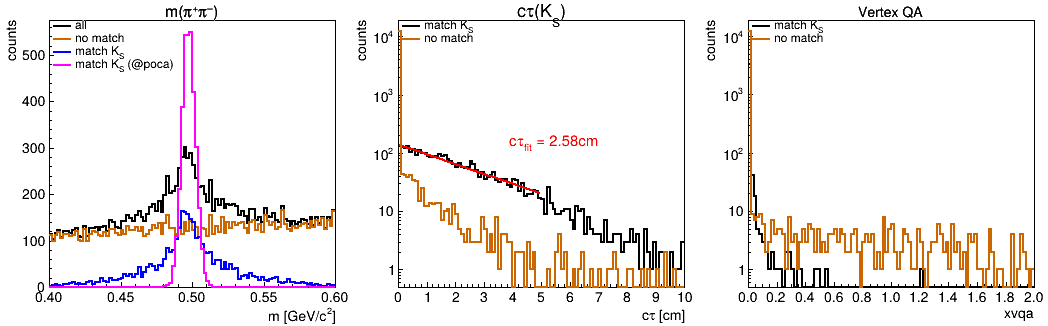
Secondary Vertex

Back to TOC

Although there is no actual vertex fitting available in HepFastSim, a simple POCA (= point of closest approach) finder is applied for all composite candidates to find the best matching decay position. Currently this only has an effect for an assumed solenoidal field parallel to the z-axis. Also, to take effect the track propagation towards the IP must be switched on.

01: # ===== Overall options ===== 
02: OPT  ;;  rndseed=123 : verbose=1 : hconf=400,3 : bzfield=1.5 : prop2ip
03: 
04: # ===== Generators ===== 
05: GEN  ;;  phsp : ecm = 4.6, 0.00965 : reaction=anti-p-,p+ : fixtarget 
06: GEN  ;;  phsp : f=0.9 : c=1 : dec = beams -> pi+ pi- pi+ pi- pi0 
07: GEN  ;;  phsp : f=0.1 : c=2 : dec = beams -> K_S0 pi+ pi- pi0 ; K_S0 -> pi+ pi-
08: 
09: # ===== Detectors ===== 
10: TRK  ;;  name = trk : ptmin=0.1  : tht=20,160 : dp=2 : dtht=1 : dphi=1 : dvtx=0.50,0.50,0.80 : dist=15
11: 
12: # ===== Trees/Reco ===== 
13: REC  ;;  dec = K_S0 -> pi+ pi- : m(K_S0)=0.4,0.6 : store(K_S0, ntp0)=cand, evt
14: 
15: # ===== Histograms ===== 
16: HIST ;;  tree=ntp0 : hist=0.4,0.6 : divx=505 : title=m(\pi^{+}\pi^{\minus});m [GeV/c^{2}] : leg=all 
17: HIST ;;  cut=!xmct : leg=no match
18: HIST ;;  cut=xmct  : leg=match K_{S}
19: HIST ;;  cut=xmct  : var=fxm : leg=match K_{S} (@poca) 
20: 
21: HIST ;;  tree=ntp0 : var=xctau : hist=0,10 : logy : cut = xmct : title=c\tau(K_{S});c\tau [cm] : leg=match K_{S}
22: HIST ;;  cut=!xmct : leg=no match
23: 
24: HIST ;;  tree=ntp0 : var=xvqa : hist=0,2 : logy : title=Vertex QA : cut=xmct : leg=match K_{S}
25: HIST ;;  cut=!xmct : leg=no match

Explanation:

• (02) : In the overall options, bzfield=1.5 : prop2ip set the solenoidal field to 1.5T, and enables track to IP propagation
• (05-07) : Generator phsp is configured to generate 2pi+ 2pi+ pi0 (90%) and KS pi+ pi- pi0 (10%) events
• (10) : Setup tracking detector with certain vertex resolution (dvtx = dvx, dvy, dvz)
• (13) : Reconstruct KS -> pi+ pi- and store TTree
• (16-19) : Invariant mass histograms of all KS candidate, w/o MC match, w/ MC match, and w/MC match propagated to common POCA.
• (21-22) : Reconstructed c·tau of matched and non matched candidates; fit of exponential finds c·tau = 2.58cm
• (24-25) : Display of vertex QA, that is the DOCA (=distance of closest approach) of track pairs forming a KS

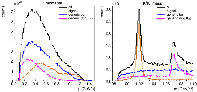
Background Study

Back to TOC

The purpose of this demo is to demonstrate the use of the generic background generation with file input to the phsp generator.

01: # ===== Overall options ===== 
02: OPT  ;;  rndseed=1 : verbose=1 : hconf=400,2 : nostat : legwid=0.38
03: 
04: # ===== Generators ===== 
05: GEN  ;;  phsp : ecm=3.0 
06: GEN  ;;  phsp : f=0.2 : c=1 : dec=beams -> phi pi+ pi- ; phi -> K+ K-  # signal 
07: GEN  ;;  phsp : f=0.6 : file=parms/dpm.dat                             # generic BG
08: GEN  ;;  phsp : f=0.2 : c=10000 : file=parms/dpm.dat : trig=K_S0       # generic BG
09: 
10: # ===== Detectors ===== 
11: TRK  ;;  name = trk : ptmin=0.1  : tht=20,160 : dp=2 : dtht=1 : dphi=1 : eff=1.0
12: 
13: # ===== Trees/Reco ===== 
14: REC  ;;  store(trk,ntp0) = evt,cand
15: REC  ;;  dec= phi -> K+ K- : store(phi,ntp1) = evt,cand
16: 
17: # ===== Histograms ===== 
18: HIST ;;  tree=ntp0 : var=xp : hist=0,1.5 : title=momenta;p [GeV/c] : leg=all : legpos=tr
19: HIST ;;  cut=chan==1 : leg=signal
20: HIST ;;  cut=chan>1 && chan<9999 : leg=generic bg
21: HIST ;;  cut=chan>9999 : leg=generic (trig K\lower[0.4]{\scale[0.7]{S}})
22: 
23: HIST ;;  tree=ntp1 : hist=0.98,1.1 : title=K^{+}K^{\minus} mass;m [GeV/c^{2}] : leg=all : legpos=tr
24: HIST ;;  cut=chan==1 : leg=signal
25: HIST ;;  cut=chan>1 && chan<9999 : leg=generic bg
26: HIST ;;  cut=chan>9999 : leg=generic (trig K\lower[0.4]{\scale[0.7]{S}})

Explanation:

• (02) : Overall options definition
• (05) : Simple setup of phsp generator with E_cm = 3 GeV
• (06) : Add signal channel phi (-> K+ K-) pi+ pi-
• (07) : Add dpm.dat as generic background source based on DPM (Dual Parton Model) generator
• (08) : Add another generic background source, but this time trigger on channels comprising a K_S
• (11) : Setup a simple tracking detector
• (14) : Store individual tracks (for momentum spectrum)
• (15) : Combinatorics for phi -> K+ K-
• (18-21) : Histogram of track momenta for the three event sources
• (23-26) : Histogram of invariant K+ K- masses for the three event sources; the bump around 1.07 GeV/c^2 is generated by pi-K mismatch from K_S decays

Using Variables

Back to TOC

As already being addressed in Configuration Setup - Using Variables it is possible to use variables per command line, which adds much more flexibility for systematic investigations without the need to provide modified configuration files all the time.

As an example let us consider the following config-file to learn the opportunities. It is a slight variation of the above background demo.

01: # ===== Overall options ===== 
02: OPT  ;;  rndseed=1 : verbose=1 : hconf=400,3 : nmc : $thtrng=20,160 : $ecm=4.6 : $frac=0.1 : ...
03:          $userhist={tree=nmc : var=p : hist=0,10 : title=gen. mom;p [GeV/c]} : $bgopt=
04: 
05: # ===== Generators ===== 
06: GEN  ;;  phsp : ecm=$ecm : reaction=anti-p-, p+ : fixtarget
07: GEN  ;;  phsp : f=$frac : c=1 : dec=beams -> phi pi+ pi- ; phi -> K+ K- # signal 
08: GEN  ;;  phsp : f=0.2 : c=10000 : file=parms/ftf_pbp.dat : $bgopt       # generic BG
09: 
10: # ===== Detectors ===== 
11: TRK  ;;  name = trk : ptmin=0.1 : tht=$thtrng : dp=2 : dtht=1 : dphi=1 : eff=1.0
12: 
13: # ===== Trees/Reco ===== 
14: REC  ;;  store(trk,ntp0) = evt,cand
15: REC  ;;  dec= phi -> K+ K- : store(phi,ntp1) = evt,cand
16: 
17: # ===== Histograms ===== 
18: HIST ;;  tree=ntp1 : hist=0.98,1.1 : title=K^{+}K^{\minus} mass;m [GeV/c^{2}] : leg=all 
19: HIST ;;  cut=chan==1   : leg=signal
20: HIST ;;  cut=chan>9999 : leg=generic bg
21: 
22: HIST ;;  $userhist

Explanation:

• (02-03) : Overall options and variables definition; we would like to control several settings per command line.
• (06-08) : Generator setup; here $ecm (energy), $frac (signal fractions) and $bgopt (options for generic events) can be modified
• (11) : Tracking detector; we want to control the polar angle coverage by $thtrng
• (23) : A complete histogram can be defined via command line.

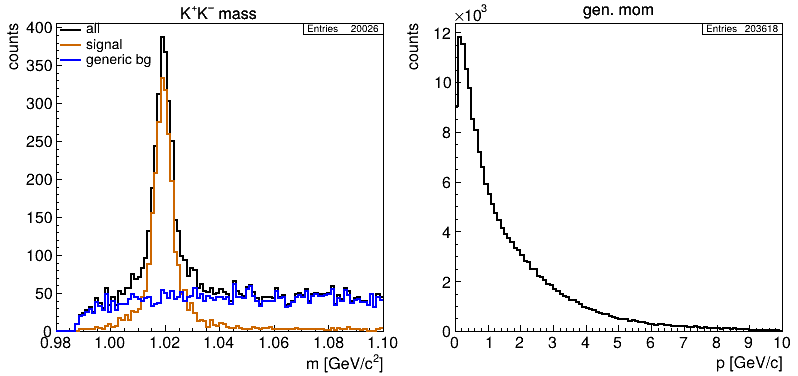
Running the simulation without additional options with HFS(20000, "cfg/demo_var.cfg") gives this effective config-file and plot as output:

GEN  ;;  phsp : ecm=4.6 : reaction=anti-p-, p+ : fixtarget
GEN  ;;  phsp : f=0.2 : c=1 : dec=beams -> phi pi+ pi- ; phi -> K+ K-
GEN  ;;  phsp : f=0.2 : c=10000 : file=parms/ftf_pbp.dat : 
TRK  ;;  name = trk : ptmin=0.1 : tht=20,160 : dp=2 : dtht=1 : dphi=1 : eff=1.0
[...]
HIST ;;  tree=nmc : var=p : hist=0,10 : title=gen. mom;p [GeV/c]

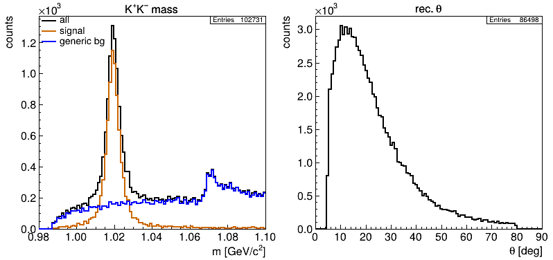
When calling as

root [9] HFS(20000, "cfg/demo_var.cfg", "$ecm=5 : $thtrng=5,80 : $bgopt=trig=K_S0 : $frac=0.2"
                    "$userhist={tree=ntp0:var=xtht*57.3:hist=0,90:title=rec. \\theta;\\theta [deg]}")

we get

GEN  ;;  phsp : ecm=5 : reaction=anti-p-, p+ : fixtarget
GEN  ;;  phsp : f=0.1 : c=1 : dec=beams -> phi pi+ pi- ; phi -> K+ K-
GEN  ;;  phsp : f=0.2 : c=10000 : file=parms/ftf_pbp.dat : trig=K_S0
TRK  ;;  name = trk : ptmin=0.1 : tht=5,80 : dp=2 : dtht=1 : dphi=1 : eff=1.0
[...]
HIST ;;  tree=ntp0:var=xtht*57.3:hist=0,180:title=;\theta [deg]

Proceed to the next section: Appendix